
Lesson 5.3 - Confidence Levels & Margins of Error
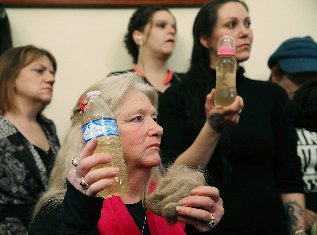
Key Question: How did researchers expose the Flint Water Crisis?
Content: Critical Values | Sample Size Calculations
Video
See the video on YouTube.
Course Resources
Resources for teaching our High School Statistics curriculum.
- Lesson Flow - timing and flow of class, using our lesson materials
- Pacing Guide - pacing our units, with daily or block schedules
- Alignment Guide - aligning our lessons to national and state standards for high school statistics
- Classroom Routines - a guidebook of classroom routines embedded within our lessons
Teaching Resources
Resources for teaching with Skew The Script.
- Discussion Norms - our model discussion norms for the classroom
- Letter to Parents - letter to share with parents about our nonpartisan approach
- Teaching Math on Civic Topics - tips for teaching math lessons that cover civic topics
Lesson Notes
Lesson-specific insights from the creators of this lesson.

In 2014, officials in Flint, Michigan changed the city's water source from the Detroit water system to the local Flint River. The move cut costs for the city. However, residents began noticing a change in their water’s color and taste. Then, they started experiencing health effects. With officials insisting the water was fine, a team of citizens and scientists gathered their own samples from the water system to make an independent determination. In this lesson, students explore how their data and methods exposed the water crisis and brought change for the city.
- Determine critical values for z-intervals
- Calculate and interpret a one-sample z-interval for a population proportion (at all confidence levels)
- Determine how changes in confidence level and sample size affect interval width
Now that students have constructed a precise 95% confidence interval for a proportion and checked the conditions for doing so (Lesson 5.2), they broaden their skillset in this lesson by constructing intervals of any confidence level (not just 95%). Specifically, students learn how to calculate different critical values to adjust the confidence level of their intervals. Then, they explore how adjusting both the critical value and the sample size affects interval width.
Familiarize yourself with the lesson materials linked above (e.g. handout, handout key, slides, video). Then, for additional background and teaching tips from the lesson creators, check out the sections below.
- To provide additional historical context for the Flint Water Crisis, briefly explain that concerns about water quality were initially dismissed by officials, and that outside researchers used statistical sampling and confidence intervals to provide evidence that the city’s water system was unsafe. This reinforces the broader idea that statistical inference can be used to investigate public claims and shed light on real issues.
- This lesson builds on the previous lesson about confidence intervals for proportions, shifting the focus toward understanding how confidence levels and sample sizes affect margins of error and interval width. Push students to think beyond the procedures of constructing confidence intervals – and toward understanding the underlying tradeoffs between confidence, variability, and precision.
- Higher confidence levels require larger critical values, which produce wider and less precise intervals. Lower confidence levels produce more precise (narrower) intervals, but with less certainty that the interval captures the true population value. Emphasizing this tradeoff with students can be helpful, as these concepts will continue to be important throughout later inference topics.
First, download this lesson's slide deck and handout key to see the prompt and sample responses for the Lesson Starter. Then, check out the additional background notes below.
Instructional routine: Would You Rather. This Lesson Starter is a modified version of the Would You Rather? instructional routine. Like the typical "Would You Rather” routine, the Lesson Starter provides a binary prompt, asking students to pick a side and defend their answer with mathematical reasoning. The main difference here is that the prompt doesn’t have the words “would you rather,” but instead asks students which of two options is most useful. Students resistant to choosing just one of the two options can be encouraged to select the option that they can best justify. There is not one correct answer to the prompt, allowing the focus to be on justification of the choice made, rather than the choice itself. You can find more background on implementing a Would You Rather here.
Purpose & Background: In this Lesson Starter, students informally consider the tradeoffs between confidence and precision when constructing confidence intervals. Is it better to be more confident but less precise, or to be less confident but more precise? Discussion will center around the temperature range, and knowing how to dress for it, in contrast to confidence that the information is correct. Considering the tradeoffs between confidence and precision in this lower stakes context (the weather) prepares students for considering the same tradeoff in the lesson’s higher stakes example: detecting lead in drinking water.
First, download this lesson's handout key and read through its Discussion Question section. Then, check out our model discussion norms and the additional background notes below.
- In general, when the null hypothesis is outside a confidence interval (i.e. the null is not a plausible value), the corresponding hypothesis test would reject it. When the null hypothesis is within a confidence interval (i.e. the null is a plausible value), the corresponding hypothesis test would fail to reject it. This relationship is true in most cases where the significance level (e.g. α = 0.05) of a two-sided hypothesis test is the complement of the confidence level (e.g. 95% confidence).
- The above relationship is not true in certain edge cases. The standard error is calculated in slightly different ways for hypothesis tests and confidence intervals. For hypothesis tests, we assume the null hypothesis is true, so we use the null hypothesized proportion value (p0) when calculating the standard error. For confidence intervals, we use the sample proportion (p̂) when calculating the standard error. If these values are very different, the relationship stated above between the hypothesis test and confidence interval is not always true. However, for the purposes of this course, students can generally assume that the relationship stated above is true.
- Just as we never fully “prove” an alternative hypothesis in a hypothesis test, this interval provides convincing evidence of the alternative hypothesis; however, it does not provide a 100% guarantee that it is true. There is always some chance (as small as it may be) that the sample gathered by researchers was unusual and that the true proportion of all homes with prominent lead levels is 10% or below.
- This lesson continues the Flint Water Crisis context from the previous lesson, but now shifts attention toward the precision of estimates (rather than simply constructing a confidence interval). The comparison between the mock study and the larger Virginia Tech study provides a natural opportunity to discuss how increased sample size reduces variability and produces narrower intervals.
- The EPA regulation discussed in the lesson states that no more than 10% of homes should exceed the lead threshold. Students sometimes interpret this as meaning that there is zero lead in the water in the rest of the homes. Clarify that the regulation concerns the proportion of homes above a specified cutoff level, rather than whether any lead is present at all.
- Students may initially believe that a narrower interval automatically provides “better” evidence. This lesson helps refine that idea by showing that interval width depends on both confidence level and sample size. Narrower intervals obtained by lowering the confidence level come at the cost of reduced confidence in the method’s long-run success rate.
- The relationship between higher sample sizes and lower spread connects directly to the law of large numbers introduced in Lesson 3.2. For example, if we flip a fair coin only twice, there is a sizable chance that 100% of the flips will be Heads. If we flip the coin 1,000 times, getting 100% Heads becomes extraordinarily unlikely. Instead, the proportion of flips that come up Heads will likely be very close to the true probability of 50%. This same idea applies to sampling distributions: as sample size increases, estimates become more tightly clustered around the true population value, producing more precise intervals.
- Distinguishing between “evidence” and “convincing evidence” can be a subtle task. A sample proportion above the EPA’s 10% threshold is certainly evidence that the true population proportion may also exceed 10%, but one sample alone may not be convincing. After all, different random samples can produce different results. Confidence intervals help students account for this uncertainty by showing a range of plausible values for the population proportion.
- Students sometimes wonder why the critical value is written as z*, rather than simply z. This is because the symbol z is reserved for z-scores. As students saw earlier in the course, z-scores can be positive or negative. In contrast, critical values (z*) are always positive. Conceptually, z* represents the number of standard errors needed to capture a desired level of confidence.
- Students may choose to memorize common critical values such as z* = 1.645 for 90% confidence, z* = 1.96 for 95% confidence, and z* = 2.576 for 99% confidence. However, it is still important for students to understand how these values are obtained using the normal curve. Encourage students to sketch the normal curve, label tail areas, and connect the confidence level to the central area of the distribution. Then, students can use technology to calculate the critical value.
Student Supports
Lesson-specific resources to support all learners.
- To support students in understanding the relationship between sample size and precision, it can help to surface the proportional reasoning that dividing by a larger number produces a smaller result, while dividing by a smaller number produces a larger result. Since sample size appears in the denominator of the standard error formula, acting as the divisor in these calculations, larger samples reduce variability in the sampling distribution.
- Vocabulary used in the context of the lesson may include words that are unfamiliar or have several meanings. In particular, the following mathematical terms may need clarification or a definition provided:
- Confidence interval
- Confidence level
- Margin of error
- Sample size
- In addition, the following contextual terms may need clarification or a definition provided:
- Environmental Protection Agency (EPA)
- Parts per billion (ppb, in reference to measured lead levels in water)
- To support students in distinguishing the term “confidence interval” from “confidence level,” encourage them to separately identify the interval endpoints, the center, the margin of error, and the confidence level before interpreting the interval in context.