
Lesson 4.2 - Sampling Distribution for a Proportion
Key Question: Can Joy's ability be used worldwide?
Content: Sampling Distribution for One Proportion
Teacher Guide
See the video on YouTube.
Part A
Activity: link
Credit: Lesson from Doug Tyson and made available by Math Medic. See the Teacher Guide Video for more info.
Course Resources
Resources for teaching our AP® Statistics curriculum.
- Lesson Flow - timing and flow of class, using our lesson materials
- Pacing Guide - pacing our units, with daily or block schedules
- CED Alignment Guide - aligning our lessons to the AP® Statistics Course and Exam Description
Teaching Resources
Resources for teaching with Skew The Script.
- Discussion Norms - our model discussion norms for the classroom
- Letter to Parents - letter to share with parents about our nonpartisan approach
- Teaching Math on Civic Topics - tips for teaching math lessons that cover civic topics
Lesson Notes
Lesson-specific insights from the creators of this lesson.
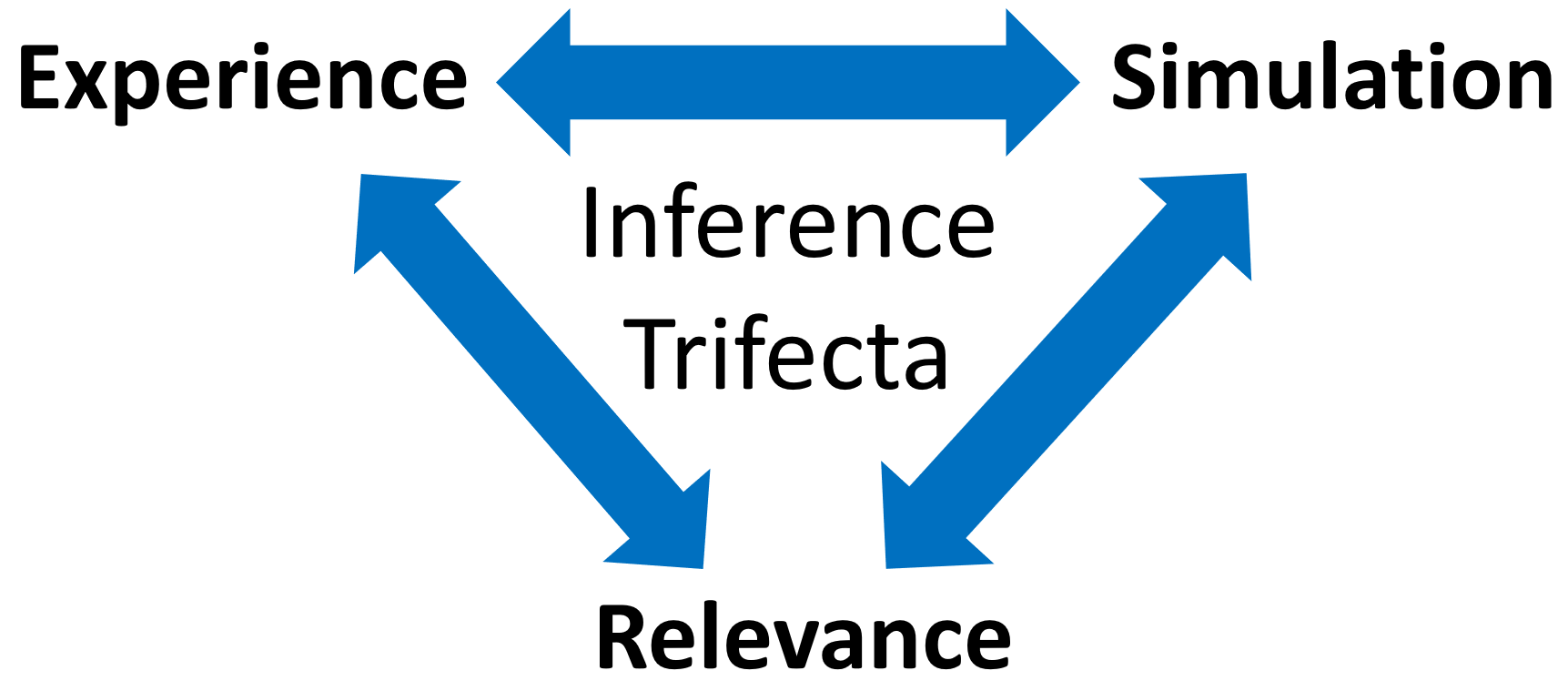
This lesson was inspired by an original activity from all-star AP Statistics instructor Doug Tyson. The lesson utilizes the inference trifecta approach, which differs from our typical lesson format. Before proceeding, watch the Teacher Guide Video and familiarize yourself with the lesson materials (e.g. handout and key). Then, for additional background and teaching tips from the lesson creators, check out the sections below.
- Use simulation to approximate the sampling distribution for a proportion
- Use the sampling distribution for a proportion to justify claims about a parameter
With this lesson, students move from general computer simulations in the last lesson (generating random maps) to simulating values for a specific parameter: the population proportion. Specifically, they use computer simulations to generate the approximate sampling distribution for a proportion. They then utilize these simulated values to evaluate whether observed results (the observed sample proportion) are unusual relative to chance results. Based on this evaluation, they make a conclusion about a claim. In performing these steps, students continue refining their approach to statistical inference, walking through the motions of conducting a hypothesis test without all the formal steps (yet). This prepares them to tackle the rest of the unit, where they’ll conduct both simulation-based and parametric (normal curve-based) hypothesis tests for a proportion.
- For daily class schedules (45-min class periods), this lesson can be completed in three days:
- Day 1: Activity from Part A (Detecting Parkinson’s with Scent)
- Day 2: Activity & Discussion from Part B (The “E-Nose”)
- Day 3: Lesson Synthesis, Practice, Mastery Check from Part B (The “E-Nose”)
- For block periods (90-minute class periods), the entire lesson can be completed in 1.5 class days.
- When used in sequence with Lesson 4.1, these activities can flow together as 4 days for daily class schedules of 2 full class days for block schedules.
- For Part A of the lesson, instructors can download the materials and view the full activity guidance at this page (from our friends at Math Medic). Note that instructors have to make a Math Medic account to download the materials. Much like Skew The Script, accounts with Math Medic are free.
- For Part B of the lesson, students complete the Amplify activity (with the instructor facilitating), as they record notes in their handout along the way. To facilitate an Amplify activity, instructors can create an Amplify account (also free) and share a single session code with their students (who can join without accounts).
- For facilitating the Amplify activity, we recommend using the “Sync to Me” pacing option. For more Amplify activity facilitation tips, check out our Amplify/Desmos session with expert Kevin McSorley.
- After the notes, students discuss the Discussion Question in small groups. Then, students discuss in full-group, with the instructor facilitating. Finally, the whole class completes the Lesson Synthesis together, before students proceed to the Practice problems and the Mastery Check.
First, download this lesson's Handout Key and read through its Discussion Question section. Then, check out our model discussion norms and the additional background notes below.
- An option for this discussion is to have students line up representing the point they chose, then to have students discuss what their positions represent. Then, have students regroup according to which outcomes are very likely, somewhat likely, etc. When discussing their groupings, it’s helpful to point out that likely and unlikely events come from both sides of the center.
- An additional regrouping can be created by asking students whether their result would provide convincing evidence that the E-Nose works. This modeling exemplifies why a simulation is useful, addressing the last portion of the Discussion Question.
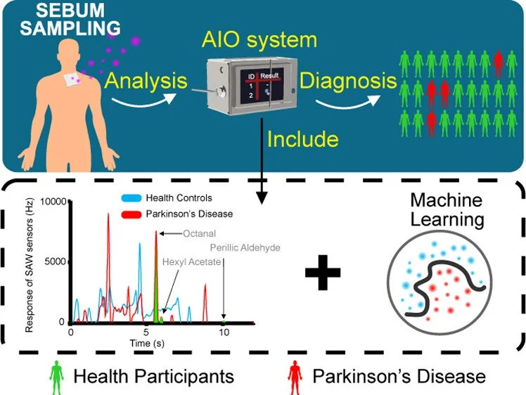
- The Zhejiang University study suggests that Parkinson’s disease is associated with a distinct chemical “fingerprint” in skin oils, likely tied to metabolic and microbiome changes – and that this signal may be detectable before clear motor symptoms appear.
- In preliminary studies, the model was able to reliably distinguish Parkinson’s patients from individuals in the control group. While this points to strong potential for early-stage, scalable screening, the approach remains in the research and validation phase, with no approved clinical devices yet. Ongoing studies are focused on confirming whether these findings hold across larger, more diverse populations before moving toward real-world use.
- Rather than jumping to the parametric formula for the sampling distribution for a proportion, which is based on a normal curve assumption, this lesson allows students to use simulation to approximate the sampling distribution. This allows students to internalize the general approach of statistical inference, without diving too early into complex formulas for exact calculations. These formulas will be introduced later in the unit, after students develop more of this early intuition.
- To support students as they begin working with calculations for the sampling distribution of a proportion, reinforce that sampling distributions are composed of many statistics, rather than many data values. This is illustrated by the graphic included in the handout showing many p̂ values, rather than dots.
Student Supports
Lesson-specific resources to support all learners.
- The language “in a world where” can provide helpful framing for interpreting sampling distributions. For example, here are several ways to use the phrase in this lesson:
- In a world where the E-Nose was randomly guessing, what is the probability that it’d get 70.8% of its guesses correct by chance alone?
- In a world where the E-Nose is randomly guessing, there is only a 2.1% probability that it’d guess 70.8% correct (or more) by chance alone.
- The sampling distribution represents all the possible trial outcomes In a world where the E-Nose was randomly guessing.
- This applet provides an excellent bridge between Part A and Part B of the lesson. The applet allows students to repeat the T-shirt experiment digitally, as well as simulate the experiment repeatedly to create a sampling distribution. Although a similar feature is also available in Part B’s Amplify activity, using the applet first provides a supportive connection to the T-shirt activity completed in class.
- Vocabulary used in the context of the lesson may include words that are unfamiliar or have several meanings. In particular, the following mathematical terms may need clarification or a definition provided:
- Population proportion
- Sample proportion
- Sampling distribution
- In addition, the following contextual terms may need clarification or a definition provided:
- Parkinson’s disease
- Sebum
- Compound
- The language “in a world where” can provide helpful framing for interpreting sampling distributions. For example: In a world where the E-Nose was randomly guessing, what is the probability that it’d get 70.8% of its guesses correct by chance alone?