
Lesson 6.3 - Least-Squares Regression
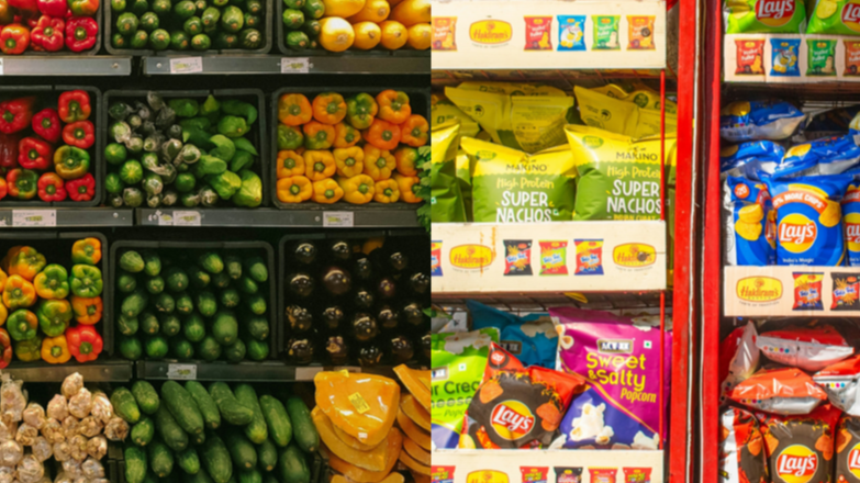
Key Question: Does access to organic foods vary by neighborhood?
Content: Least-Squares | Interpreting Slope & y-Intercept | Coefficient of Determination (r²)
Video
Course Resources
Resources for teaching our High School Statistics curriculum.
- Lesson Flow - timing and flow of class, using our lesson materials
- Pacing Guide - pacing our units, with daily or block schedules
- Alignment Guide - aligning our lessons to national and state standards for high school statistics
- Classroom Routines - a guidebook of classroom routines embedded within our lessons
Teaching Resources
Resources for teaching with Skew The Script.
- Discussion Norms - our model discussion norms for the classroom
- Letter to Parents - letter to share with parents about our nonpartisan approach
- Teaching Math on Civic Topics - tips for teaching math lessons that cover civic topics
Lesson Notes
Lesson-specific insights from the creators of this lesson.
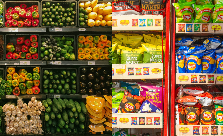
A former Skew The Script student noticed that her local grocery store offered fewer organic items than another location – from the same company – in a wealthier part of town. So, she collected data from every location in the city to investigate. In this lesson, students analyze this data set using least-squares regression, as they model the trend between income and access to organic foods. Then, they consider the fairness of this trend, both from the consumers’ perspective and from the company’s perspective.
- Describe how least-squares regression line (LSRL) models are fit to data
- Interpret the slope and y-intercept of an LSRL model
- Determine and interpret the coefficient of interpretation (r²)
In the previous lessons of this unit, students used and interpreted linear regression models, without addressing the underlying mechanics of how these models were fit to real data sets. In this lesson, these underlying mechanics are demystified, as students explore the least-squares method for fitting regression lines. By exploring visualizations created with technology (CODAP), students refine their interpretations of the characteristics of the least-square regression line (LSRL). These refined understandings include more precise interpretations of the components of linear models (slope and y-intercept) and using the coefficient of determination (r²) to describe model strength. In the next lesson, students will use CODAP themselves to create their own regression models from raw data.
Before proceeding: Familiarize yourself with the lesson materials linked above (e.g. handout, handout key, slides, video). Then, for additional background and teaching tips from the lesson creators, check out the sections below.
- It’s helpful to emphasize that this data set was gathered by a real high school student who used her learning in statistics class to investigate a topic that she cared about. Although much of this course is about getting students to think critically as data consumers, telling this story can help students see themselves as data gatherers and producers too. This framing is especially helpful as students approach the capstone project in Unit 7 or, more importantly, any data projects they perform in college, the workforce, or on their own.
- Instead of using the provided San Antonio data set in the lesson, instructors can consider gathering their own data set that reflects the relationship between income and access to organic foods in their own region. Income data is accessible via the US Census. Grocery data can be more difficult to gather, and its accessibility varies by region. However, the best strategy is to go to the website of the most popular grocery chain in your region. Then, on the webpage for each store location, perform a search for the products offered in-store. See if there is an “organic” filter for the search results. If so, click the filter and search for all products flagged as organic. The number of total results that appear is the number of organic items offered in store.
- To find the LSRL from raw data, technology such as CODAP should be used. The focus in this lesson should be for students to be able to identify and interpret the slope, y-intercept, r, and r² values from regression output, rather than doing the calculations manually themselves.
- If time allows, we highly recommend showing students the optional video that explains some of the mathematical background behind the coefficient of determination (r²). The explanation in the video helps motivate the interpretation of r², so that the interpretation becomes meaningful to students – rather than another memorized sentence stem.
First, download this lesson's slide deck and handout key to see the prompt and sample responses for the Lesson Starter. Then, check out the additional background notes below.
Instructional routine: Which One Doesn't Belong. The Which One Doesn’t Belong (WODB) routine is often a student favorite. Students are presented with four images or expressions, and they determine which option does not belong. The key to this routine is in the explanation from students. Because all options could be selected and justified, the reasoning and ability to communicate their choice is what’s important. These are low floor, high ceiling problems that allow for all students to engage. You can find more background on implementing this routing here.
Purpose & Background: This Lesson Starter is designed to resurface what students already know about lines and their equations. Three of the options (A, C, & D) describe the same linear function. For this reason, Option B may seem like a natural choice for the one that doesn’t belong. However, there are many other ways to decide how one of the options doesn’t belong, often using simpler criteria (e.g. Option A doesn’t belong because it’s the only graph). Instructors can use student responses to formatively assess their understanding of linear functions, in preparation for jumping into exploration of equations for least squares regression lines (LSRLs) in the lesson.
First, download this lesson's handout key and read through its Discussion Question section. Then, check out our model discussion norms and the additional background notes below.
- It can be helpful to mention that the y-variable does not describe the volume of organic products in the store (i.e. it’s not the stock or raw number of organic items on shelves). Rather, the y-variable describes the number of organic product types or varieties. Therefore, when there are fewer organic items, this means that there are fewer organic choices for consumers.
- One way to frame this discussion is as a trade off between groups and individuals. If one group tends to buy more organic than another group, they get more organic varieties offered at their stores. However, all groups will likely have some individuals who would prefer to buy organic. Because of where they live, these individuals may have to spend more time (especially if using public transit) and money (gas or transit fare) to buy their products elsewhere.
- On the other hand, offering more varieties of organic items could be costly for the store. Stocking additional types of products could mean having to develop new supply chains, track new product-specific expiration and care instructions, etc. The company may need to sell a certain volume of a product in order to make offering it worth the cost.
- The grocery store data set was gathered by an actual high school student, who used her learning in statistics class to investigate a topic that she cared about. Sharing this background can help inspire students to take the initiative to gather their own data about their own areas of interest. Students can also consider gathering income and grocery data within their own city or region as their Unit 7 capstone project.
- The student gathered the data in 2019. She found the average household income in each zip code from this US census aggregator. She found the food data by searching H-E-B’s website. Specifically, she went to the webpage for each full-size store in the city of San Antonio. On each store’s webpage, she searched for products offered in-store that were flagged as “organic.” The data set shows the total number of returned search results for each store.
- It’s worth noting for students that the average household income in the data set is coded in terms of thousands of dollars (e.g. a value of 53 indicates $53,000). This creates an opportunity to discuss how units affect the interpretation of slope.
- Why do we square the residuals to get rid of negatives? Why not just find the model that minimizes the absolute value of the residuals? There are two central reasons for this:
- i) Squaring emphasizes larger differences, which can be helpful for surfacing outliers.
- ii) Squares often have nicer mathematical properties than absolute values. In particular, finding the model that minimizes the residual error often means performing a derivative. It’s much easier to find the derivative of a square than an absolute value. Finding derivatives is what some software platforms do in the background to find the LSRL.
- The coefficient of determination (r²) alone does not provide enough information to fully determine the correlation coefficient (r). The magnitude can be recovered algebraically, but the sign must be determined from the direction of the relationship seen in the scatterplot. This provides another reason to examine the graph before relying solely on summary statistics.
- The interpretation of r² introduces the important idea that statistical models explain some variation in a response variable, but rarely all of it. Consider showing students the optional video that explains some of the mathematical background behind the interpretation of r².
Student Supports
Lesson-specific resources to support all learners.
- Mathematical Language Routines useful for this lesson: Collect and Display (MLR2) – As students' prior learning for linear functions is resurfaced, this lesson is a good place to begin a visual reference for the vocabulary students are expected to use. As students progress through this lesson and the next, capture these terms in a publicly displayed collection in class, adding to the collection throughout the unit.
- Vocabulary used in the context of the lesson may include words that are unfamiliar or have several meanings. In particular, the following mathematical terms may need clarification or a definition provided:
- Residual
- Squared
- Slope
- y-intercept
- Positive and negative associations
- Strong and weak associations
- Coefficient of determination
- In addition, the following contextual terms may need clarification or a definition provided:
- Organic
- Access
- Zip code
- Low income and high income
- In class conversation, it can be helpful to describe the magnitude of the slope as the steepness of the line and describe the magnitude of r or r² as the strength of the relationship. Consider also showing students examples of steep lines with weak relationships (steep lines with data spread out far from the line) and shallow lines with strong relationships (almost flat lines with data closely hugging the line). This will not only help students refine their language when discussing steepness versus strength, but it will also help them conceptually differentiate the meaning of a high magnitude slope value (steep line) from the meaning of a high magnitude r or r² value (data values close to line).