Lesson 2.A.1 - Describing Two Categorical Variables (Version A)

Key Question: Is stop and frisk discriminatory?
Content: Joint, Marginal, & Conditional Frequencies | Side-By-Side Bar Charts, Segmented Bar Charts, & Mosaic Plots
Alignment: CED Topic 2.1-2.2
Video
Course Resources
Resources for teaching our AP® Statistics curriculum.
- Lesson Flow - timing and flow of class, using our lesson materials
- Pacing Guide - pacing our units, with daily or block schedules
- CED Alignment Guide - aligning our lessons to the AP® Statistics Course and Exam Description
Teaching Resources
Resources for teaching with Skew The Script.
- Discussion Norms - our model discussion norms for the classroom
- Letter to Parents - letter to share with parents about our nonpartisan approach
- Teaching Math on Civic Topics - tips for teaching math lessons that cover civic topics
Lesson Notes
Lesson-specific insights from the creators of this lesson.
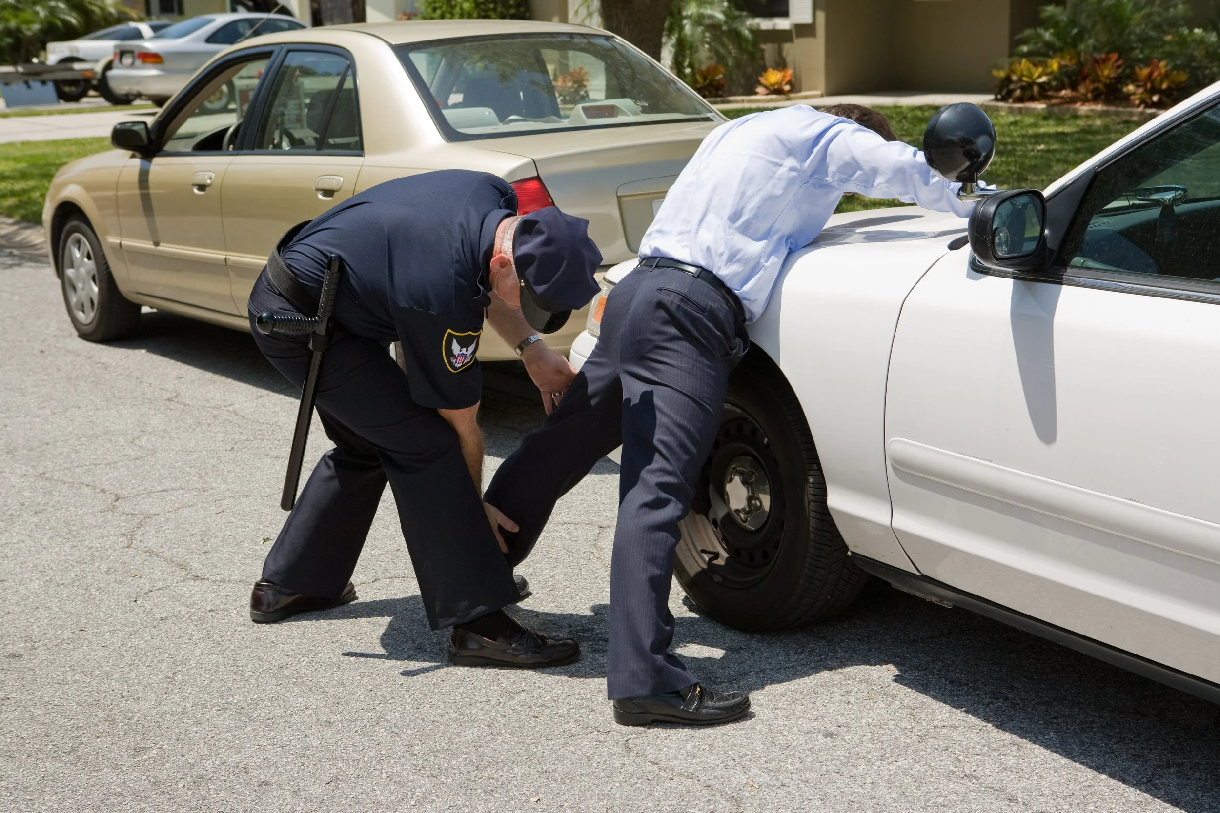
This lesson explores public data from stop and frisk – a New York City program in which police stop individuals on the street if they have reasonable suspicion that a crime has been, is being, or is about to be committed. Rather than reactionary policing – in which officers respond to crimes already being committed – a goal of stop and frisk is to proactively prevent more crime. However, some city residents allege that police discriminate in terms of who they choose to stop. In this lesson, students use marginal distributions, conditional distributions, and data visuals to investigate.
- Calculate and interpret joint, marginal, and conditional relative frequencies
- Interpret side-by-side bar charts, segmented bar charts, and mosaic plots
- Describe associations between two categorical variables
Before proceeding: Familiarize yourself with the lesson materials linked above (e.g. handout, handout key, slides, video). Then, for additional background and teaching tips from the lesson creators, check out the sections below.
- It’s important to provide a nonpartisan framing for the lesson context. In particular, it’s important to share that the intent of stop and frisk is to provide a more proactive model of policing that can prevent more crime, rather than the typical reactionary model in which officers respond to calls of crimes already being committed. In addition, some residents allege that police discriminate in terms of how they apply reasonable suspicion and who they choose to stop. The goal of the analysis is to use detailed public data from the program to investigate these claims.
- There are various statistical approaches to analyzing discrimination, many of which use methods beyond the scope of this lesson. To keep the conversation focused, it’s helpful to center the analysis specifically on Mayor Bloomberg’s claim: “...we put all the cops in the minority neighborhoods. Yes, that's true. Why'd we do it? Because that's where all the crime is.” The methods in this lesson can provide insight on whether this specific claim is supported by the stop and frisk data set.
- Another way to keep conversations focused is to refer back to a concept from earlier in the course: generalizability. Stop and frisk is a particular model of policing. Patterns we find in stop and frisk data may not be generalizable to other methods of policing. In addition, patterns we find in New York City data may not generalize to other regions. So, we should be careful about claims that attempt to generalize findings from this data set to other policing contexts.
- This lesson covers a relatively high number of statistical ideas and methods. Pointing out connections between them can help students better internalize them. For example, vertically stacking the bars in a side-by-side bar chart would yield a segmented bar chart. In addition, adjusting the bar widths in a segmented bar chart (according to sample sizes) would yield a mosaic plot. So, side-by-side bar charts, segmented bar charts, and mosaic plots are highly interrelated.
First, download this lesson's Handout Key and read through its Discussion Question section. Then, check out our model discussion norms and the additional background notes below.
- The discussion provides a good opportunity to promote deeper conceptual understanding of the mosaic plot. Have students take a look at the size of the areas in the mosaic plot. Just as 88.4% of stops that found crime were stops of Black and Hispanic individuals, 88.4% of the “crime found” area in the mosaic plot is contained within the Black and Hispanic columns. However, this high share of stops that found crime isn’t driven by the height of those columns (the crime rates). After all, the heights (crime rates) are similar among each group. Rather, it’s driven by the differences in column widths. So, this pattern is more attributable to the rates at which each group was stopped, rather than the rates at which each group committed crimes.
- Another connection is the similarity of the marginal and conditional relative frequencies. 88.5% of all police stops were stops of Black and Hispanic individuals (marginal relative frequency). Similarly, 88.4% of stops that found crime and 88.5% of stops that did not find crime were stops of Black and Hispanic individuals (conditional relative frequencies). The similarity between the marginal and conditional relative frequencies suggests that the rate at which each group is stopped, rather than the crime rate among each group, is the main driver of the trends we see.
- It’s worth noting that the data from this lesson can’t definitively prove or disprove Bloomberg’s claims. For example, the rates of crime discovered by police stops may differ from the rates of undiscovered (but still real) crime. Still, the mayor made these claims during a speech on stop and frisk, and this data from the program (without making outside assumptions) falls short of supporting those claims.
- The legal backing for stop and frisk comes from Terry v Ohio (1968), which held that police can stop individuals if they have “a reasonable suspicion that a crime has been, is being, or is about to be committed by the suspect.” This is a lower threshold than the traditional "probable cause" criteria. So, police have to use their training and discernment to determine if there’s reasonable suspicion that a crime is “about to be committed.” According to proponents, this allows police to be more proactive, preventing crime rather than merely responding to it. However, critics claim that this level of leeway for stops is where bias can arise. Terry stops, as they’re known from the Terry case, occur in a variety of areas nationwide.
- The stop and frisk data is recorded by police officers. In addition to police-recorded data, researchers also sometimes utilize data gathered from individuals’ reporting of their interactions with police, such as the Police-Public Contact Survey.
- The coding of racial groups from the stop and frisk data set was done in a consistent manner to other research on stop and frisk: black and black-hispanic individuals were coded as "Black," white-hispanic individuals were coded as “Hispanic," white non-hispanic individuals were coded as “White,” and all other categories were coded exactly as written in the original data set (Asian, Middle Eastern, Native American). The Middle Eastern and Native American groups did not have a high enough sample size for this analysis; however, information for these groups can be found in the full data set. A file showing our full data analysis methodology can be downloaded here.
- At this point in the course, we say that two categorical variables are “associated” if conditional relative frequencies differ between groups. Later in the course, we’ll use hypothesis tests to determine if these associations are statistically significant (so large that they’re unlikely due to chance alone). This provides a more formal threshold for determining whether two variables are truly “associated” with one another. For the data set in this lesson, a chi-square test for independence yields a p-value of 0.353. So, the association between race and crime rates is not statistically significant.
- There are multiple ways to make visualizations of categorical data misleading. These include using pictures in place of bars for bar graphs or using truncated y-axes. Check out our Classic AP Stats 1.1 Lesson (created before the 2026 course revision) or High School Statistics Lesson 1.1 for examples. Note that misleading graphs are not covered in the current AP Statistics Course and Exam Description.
Student Supports
Lesson-specific resources to support all learners.
- For supporting students with finding conditional distributions, encourage them to cover up any parts of the two-way table they no longer have to consider. For example, in the practice exercise in which students are asked to “calculate the conditional distribution of severity of symptoms for Medicine A,” students can use their hand to cover any table cells that don’t apply to Medicine A. This makes it clearer for students that the new total for their fractions is just the total among the Medicine A cases.
- Vocabulary used in the context of the lesson may include words that are unfamiliar or have several meanings. In particular, the following mathematical terms may need clarification or a definition provided:
- Two-Way Table / Contingency Table
- Joint Relative Frequency
- Marginal Relative Frequency
- Side-by-Side Bar Chart
- Conditional Relative Frequency
- Segmented Bar Chart
- Mosaic Plot
- Weighted average
- In addition, the following contextual terms may need clarification or a definition provided:
- Police Stop