
Lesson 3.B.5 - Chi-Square Test for Independence
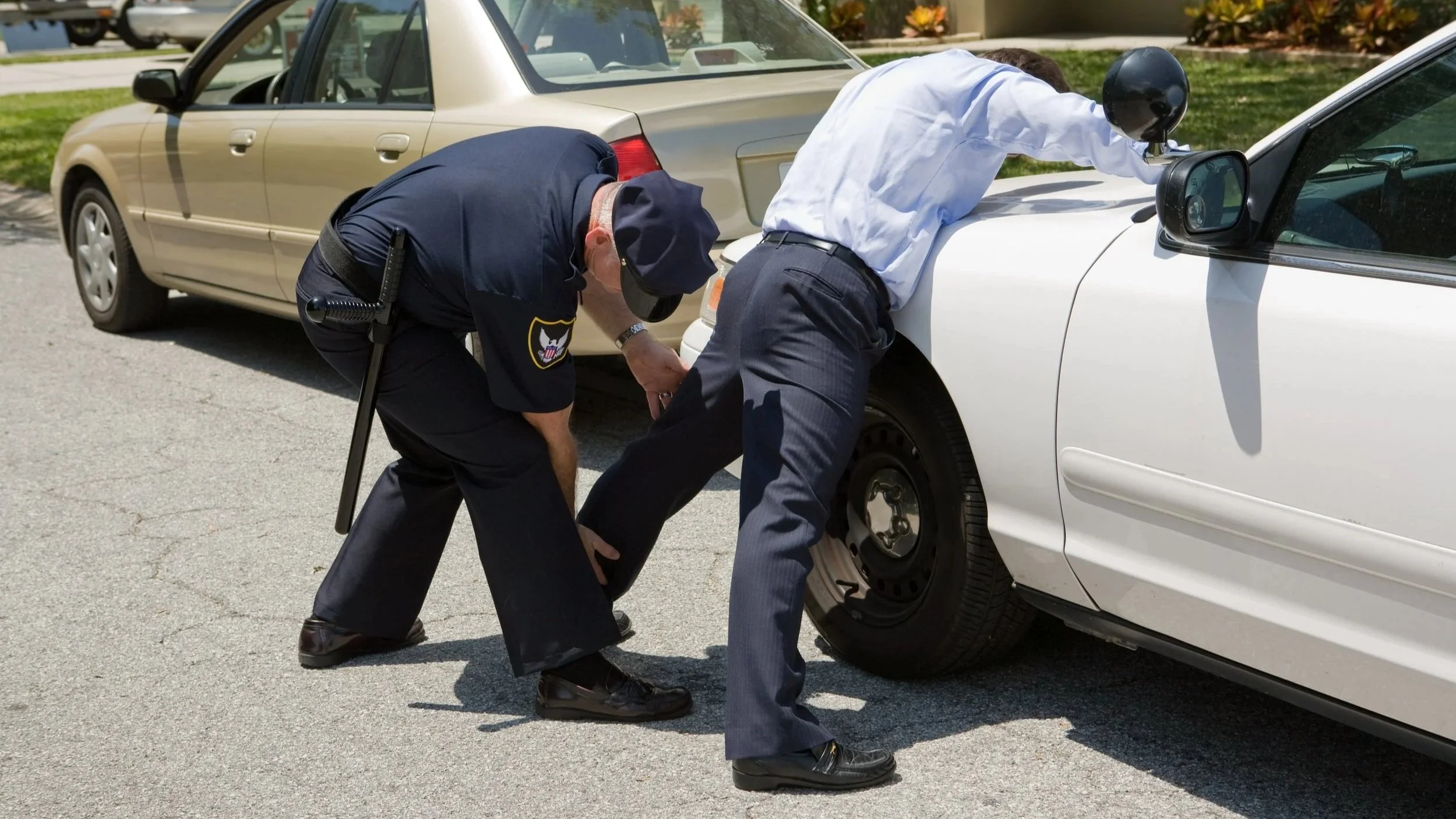
Key Question: Among cooperative individuals, is police use of force associated with race?
Content: Chi-Square Test for Independence | Degrees of Freedom | Conditions
Alignment: CED Topics 3.14-3.15
Video
See the video on YouTube.
Course Resources
Resources for teaching our AP® Statistics curriculum.
- Lesson Flow - timing and flow of class, using our lesson materials
- Pacing Guide - pacing our units, with daily or block schedules
- CED Alignment Guide - aligning our lessons to the AP® Statistics Course and Exam Description
Teaching Resources
Resources for teaching with Skew The Script.
- Discussion Norms - our model discussion norms for the classroom
- Letter to Parents - letter to share with parents about our nonpartisan approach
- Teaching Math on Civic Topics - tips for teaching math lessons that cover civic topics
Lesson Notes
Lesson-specific insights from the creators of this lesson.

New York City’s stop and frisk program allows police to stop individuals on the street if they have reasonable suspicion that a crime has been, is being, or is about to be committed. Using 2003 – 2013 data from the program, a Harvard researcher found evidence that even among “perfectly compliant” individuals (not arrested, not carrying criminal items, not evasive, and cooperated with directions), police sometimes used force – and they used force at a significantly higher rate on Black and Hispanic individuals, compared to White individuals. After a 2020 executive order from the governor, New York City created the Police Reform and Reinvention Collaborative Plan. In the years since, has there been a detectable change in the stop and frisk program? In this lesson, students use more recent data from the program to investigate.
- Determine whether to use a chi-square test for homogeneity or independence
- Check conditions and calculate degrees of freedom for a chi-square test
- Conduct a chi-square test for independence
Before proceeding: Familiarize yourself with the lesson materials linked above (e.g. handout, handout key, slides, video). Then, for additional background and teaching tips from the lesson creators, check out the sections below.
- It’s important to provide a nonpartisan framing for the lesson context. In particular, it’s important to share that the intent of stop and frisk is to provide a more proactive model of policing that can prevent more crime, rather than the typical reactionary model in which officers respond to calls of crimes already being committed. In addition, some residents allege that police discriminate in terms of how they apply reasonable suspicion and who they choose to stop. The goal of the analysis is to use detailed public data from the program to investigate these claims.
- There are various statistical approaches to analyzing discrimination, many of which use methods beyond the scope of this lesson. To keep the conversation focused, it’s helpful to center the analysis specifically on this question from the lesson: “Among fully cooperative individuals, is there convincing statistical evidence that police use of force is associated with race?”
- When distinguishing between chi-square tests for homogeneity and independence, emphasize the structure of the data collection (rather than relying only on keywords in the question). For independence, one sample is used to examine the relationship between two categorical variables; for homogeneity, one categorical variable is compared across multiple samples or groups. Asking students to identify what was sampled and what was measured can help them reason to the appropriate test, rather than memorize a decision rule.
First, download this lesson's Handout Key and read through its Discussion Question section. Then, check out our model discussion norms and the additional background notes below.
- The Discussion Question pushes students to think carefully about how we define the population of interest. Among fully cooperative individuals who were stopped by police, there is not convincing evidence that the rate of recorded force is associated with race. However, this does not answer the broader question of whether race is associated with the rates at which New York City residents, in general, experience police use of force. In terms of this broader population, Black and Hispanic residents may be more likely to experience force, since they are more likely to be stopped and have interactions with police in the first place.
- Imagine repeating this analysis, but with a random sample among all New York City residents who would be fully cooperative if stopped by police. In addition, imagine expanding the categories for police interactions to the following:
- Never stopped by police
- Stopped and no force used
- Stopped and force used
- In the above case, there may be a statistically significant association. White individuals may be less likely to be stopped and, therefore, may be less likely to experience force than Black and Hispanic individuals. However, practically speaking, such a study would be difficult to implement. The population of individuals who “would be fully cooperative if stopped by police” is hard to define, since it would require making predictions about individuals’ behavior in a hypothetical scenario of being stopped by police officers.
- The legal backing for stop and frisk comes from Terry v Ohio (1968), which held that police can stop individuals if they have “a reasonable suspicion that a crime has been, is being, or is about to be committed by the suspect.” This is a lower threshold than the traditional “probable cause” criteria. So, police have to use their training and discernment to determine if there’s reasonable suspicion that a crime is “about to be committed.” According to proponents, this allows police to be more proactive, preventing crime rather than merely responding to it. However, critics claim that this level of leeway for stops is where bias can arise. Terry stops, as they’re known from the Terry case, occur in a variety of areas nationwide.
- The stop and frisk data is recorded by police officers. In addition to police-recorded data, researchers also sometimes utilize data gathered from individuals’ reporting of their interactions with police, such as the Police-Public Contact Survey.
- The coding of racial groups from the stop and frisk data set was done in a manner consistent with other research on stop and frisk: black and black-Hispanic individuals were coded as "Black," white-Hispanic individuals were coded as “Hispanic," white non-Hispanic individuals were coded as “White,” and all other categories were coded exactly as written in the original data set (Asian, Middle Eastern, Native American). The Asian, Middle Eastern, and Native American groups did not have a high enough sample size for this analysis; however, information for these groups can be found in the full data set.
- Although chi-square may look somewhat different from the inference procedures students have encountered previously, the underlying reasoning is familiar: describe what we would expect under the null hypothesis, measure how far the observed data depart from that expectation, and determine whether such a discrepancy could reasonably occur by chance. Reinforcing this common structure across inference procedures can help students focus on the statistical reasoning that connects them, rather than treating each new test as a separate procedure to memorize.
- The chi-square distribution is right-skewed. Larger chi-square values fall further into the right tail, leaving less area to the right. This corresponds to a smaller p-value and stronger evidence against the null hypothesis. For a more detailed look at how the p-value for a chi-square test is calculated from a chi-square distribution, check out this supplemental video.
- Degrees of freedom determine the shape of the chi-square distribution used to calculate the p-value. With fewer degrees of freedom, the distribution is strongly right-skewed; as degrees of freedom increase, the distribution becomes more symmetric and increasingly resembles a normal distribution. This connects to familiar ideas about standardization and the Central Limit Theorem: each chi-square contribution \( \frac{(\text{observed} - \text{expected})^2}{\text{expected}} \) can be thought of as a squared, standardized discrepancy between an observed and expected count, similar in structure to a squared z-score: \( \left(\frac{x - \mu}{\sigma}\right)^2 \). The chi-square statistic combines these contributions across the table, and as the degrees of freedom increase, the distribution of this combined measure becomes increasingly normal in shape.
Student Supports
Lesson-specific resources to support all learners.
- When deciding between a chi-square test for independence and homogeneity, encourage students to begin with the study design, rather than the name of the test. One sample with two categorical variables calls for a test for independence, while multiple samples or groups with one categorical variable call for a test for homogeneity.
- The 10% condition plays the same role here that it has in earlier inference procedures: when sampling without replacement, it allows observations in the sample to be treated as approximately independent. Explicitly reconnecting this condition to earlier inference procedures can reinforce that chi-square is using familiar statistical principles in a new setting.
- Vocabulary used in the context of the lesson may include words that are unfamiliar or have several meanings. In particular, the following mathematical terms may need clarification or a definition provided:
- Independence / independent
- Homogenity
- Degrees of freedom
- Association
- In addition, the following contextual terms may need clarification or a definition provided:
- Stop and frisk
- Reasonable suspicion
- Probable cause
- Fully cooperative