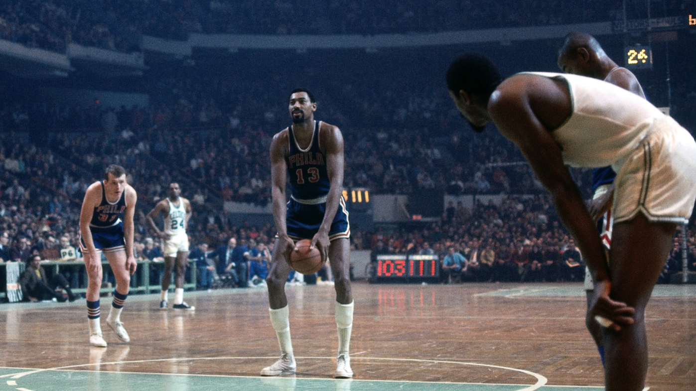
• Playing the videos (embedded in the lesson slide deck) of Wilt Chamberlain shooting free throws overhanded and underhanded helps motivate the lesson in two key respects:
• It helps students who are less familiar with basketball see what “granny style” free throws look like
• It provides a natural entry point for modeling free throws with a binomial distribution. Because the player stands a fixed distance away from the hoop and the other team is not allowed to guard them, each shot can be considered an identical and independent trial.
• Students often ask why BINS includes both “independence” and “same probability,” since these can feel redundant. Emphasize that the former is about whether trials impact one another, while the latter is about the numerical value of p. For example, imagine a player shooting a free throw and, on the next play, shooting a layup (a shot close to the hoop). Their performance on the last play’s free throw may not influence their probability of making the next play’s layup. So, we could say that these trials are independent. However, the probability of making a layup is different from the probability of making a free throw. So, they don’t have the same probability. Therefore, the “I” of BINS would be satisfied, but the “S” would not.
• It can be helpful to encourage students to interpret binomial probabilities in context, using language such as “the probability of getting exactly 7 successful free throws out of 10 attempts.” Reinforcing this connection between the number of successes and the total number of trials supports clearer understanding and communication.

First, download this lesson's Handout Key and read through its Discussion Question section. Then, check out our model discussion norms and the additional background notes below.

• To this day, when googling “the best free throw shooter ever,” the first results tend to be Stephen Curry, Steve Nash, and Mark Price. There’s no mention of Elena Delle Donne, whose career free throw percentage (as shown in the lesson slides and video) is several points higher than anyone in the entire history of the men’s league. In addition, the conditions for free throws are almost identical between the leagues, as the NBA and WNBA have identical hoop heights and free throw line distances. The only difference is that the NBA has a slightly larger ball. Still, the lack of recognition for Donne is remarkable.
• Our calculations assume that Wilt’s probability of making free throws “granny style” would stay at 61.3% throughout his entire career. For most players, free throw accuracy actually tends to increase over time, as they get accustomed to the game pressure and refine their shooting mechanics. Because Wilt’s granny style season was early in his career, it’s plausible that if he had stuck with the technique, he would have refined it further and shot at a higher than 61.3% accuracy in later seasons.
• Consider asking students whether switching to underhanded (“granny style”) free throws might improve performance for more players. What evidence would they want to collect to evaluate this claim?

• To further illustrate the idea of a fixed number of trials, consider comparing a “best of ten” free throw contest with a sudden-death format, in which the first player to make 5 shots wins. Ask students to determine which scenario fits a binomial setting (the first one), and to explain why the other does not.
• If it doesn’t arise organically, consider surfacing the idea that – while free-throws are often modeled as independent with a constant probability of success – factors such as fatigue and game pressures mean that day-to-day performances vary. This can help students understand that statistical models are approximations, even in seemingly controlled situations.
• As optional extensions, consider sharing this article on the science of free throw technique, or this short article about the Guinness World Record holder for most consecutive free throws.

• Optional videos are provided on deriving the binomial coefficient and the standard deviation for the binomial in this supplementary playlist.
• It’s worth noting that a binomial distribution is a function in which the input is the number of successes, x, and the output is the probability of observing that value. The parameters, n and p, remain fixed for a given situation. Like any function, a binomial distribution can be represented algebraically using a formula, numerically with a probability distribution table, or graphically with a histogram.
• Although outside the scope of this course, students who have studied the binomial theorem in Algebra 2 may recognize the identical structure in binomial probability calculations. Another mathematical connection can be drawn between the binomial coefficient and Pascal’s triangle. Check out this video for an exploration of these connections.
• In lesson 2.B.1, students were introduced to the formula for expected value of a discrete probability distribution. Since the binomial is also discrete, some students may wonder why its expected value formula appears to be different. A useful extension is to have students construct a probability distribution table for a small value of n (for example, n=5) and compute the expected value using the general formula. This helps to illustrate that the result, np, is a simplified form that applies specifically to binomial distributions. For students seeking an additional challenge, consider exploring why this simplification holds in general.
• Looking ahead, binomial distributions lay the foundation for sampling distributions. The sampling distribution of a proportion is built from repeated independent trials with a constant probability of success, mirroring a binomial setting. Supplementary material is provided in later units of the course to help draw this connection.